Machine Learning #1 : 분류 문제 - Logistic 회귀
자료 출처 : Datacampus "빅데이터 분석기사 자격증 과정 실기" 책 예제 : https://www.datacampus.co.kr/board/read.jsp?id=98394&code=notice
data/ library import
In [135]:
import warnings
In [136]:
warnings.filterwarnings('ignore')
In [3]:
import pandas as pd

data= pd.read_csv('breast-cancer-wisconsin.csv')
data 확인
In [4]:
data.head()
Out[4]:
| code | Clump_Thickness | Cell_Size | Cell_Shape | Marginal_Adhesion | Single_Epithelial_Cell_Size | Bare_Nuclei | Bland_Chromatin | Normal_Nucleoli | Mitoses | Class | |
|---|---|---|---|---|---|---|---|---|---|---|---|
| 0 | 1000025 | 5 | 1 | 1 | 1 | 2 | 1 | 3 | 1 | 1 | 0 |
| 1 | 1002945 | 5 | 4 | 4 | 5 | 7 | 10 | 3 | 2 | 1 | 0 |
| 2 | 1015425 | 3 | 1 | 1 | 1 | 2 | 2 | 3 | 1 | 1 | 0 |
| 3 | 1016277 | 6 | 8 | 8 | 1 | 3 | 4 | 3 | 7 | 1 | 0 |
| 4 | 1017023 | 4 | 1 | 1 | 3 | 2 | 1 | 3 | 1 | 1 | 0 |
In [5]:
data.info()
<class 'pandas.core.frame.DataFrame'>
RangeIndex: 683 entries, 0 to 682
Data columns (total 11 columns):
 #   Column                       Non-Null Count  Dtype
---  ------                       --------------  -----
 0   code                         683 non-null    int64
 1   Clump_Thickness              683 non-null    int64
 2   Cell_Size                    683 non-null    int64
 3   Cell_Shape                   683 non-null    int64
 4   Marginal_Adhesion            683 non-null    int64
 5   Single_Epithelial_Cell_Size  683 non-null    int64
 6   Bare_Nuclei                  683 non-null    int64
 7   Bland_Chromatin              683 non-null    int64
 8   Normal_Nucleoli              683 non-null    int64
 9   Mitoses                      683 non-null    int64
 10  Class                        683 non-null    int64
dtypes: int64(11)
memory usage: 58.8 KB
In [7]:
data.describe().transpose()
Out[7]:
| count | mean | std | min | 25% | 50% | 75% | max | |
|---|---|---|---|---|---|---|---|---|
| code | 683.0 | 1.076720e+06 | 620644.047655 | 63375.0 | 877617.0 | 1171795.0 | 1238705.0 | 13454352.0 |
| Clump_Thickness | 683.0 | 4.442167e+00 | 2.820761 | 1.0 | 2.0 | 4.0 | 6.0 | 10.0 |
| Cell_Size | 683.0 | 3.150805e+00 | 3.065145 | 1.0 | 1.0 | 1.0 | 5.0 | 10.0 |
| Cell_Shape | 683.0 | 3.215227e+00 | 2.988581 | 1.0 | 1.0 | 1.0 | 5.0 | 10.0 |
| Marginal_Adhesion | 683.0 | 2.830161e+00 | 2.864562 | 1.0 | 1.0 | 1.0 | 4.0 | 10.0 |
| Single_Epithelial_Cell_Size | 683.0 | 3.234261e+00 | 2.223085 | 1.0 | 2.0 | 2.0 | 4.0 | 10.0 |
| Bare_Nuclei | 683.0 | 3.544656e+00 | 3.643857 | 1.0 | 1.0 | 1.0 | 6.0 | 10.0 |
| Bland_Chromatin | 683.0 | 3.445095e+00 | 2.449697 | 1.0 | 2.0 | 3.0 | 5.0 | 10.0 |
| Normal_Nucleoli | 683.0 | 2.869693e+00 | 3.052666 | 1.0 | 1.0 | 1.0 | 4.0 | 10.0 |
| Mitoses | 683.0 | 1.603221e+00 | 1.732674 | 1.0 | 1.0 | 1.0 | 1.0 | 10.0 |
| Class | 683.0 | 3.499268e-01 | 0.477296 | 0.0 | 0.0 | 0.0 | 1.0 | 1.0 |
In [11]:
data.columns.tolist()
Out[11]:
['code',
 'Clump_Thickness',
 'Cell_Size',
 'Cell_Shape',
 'Marginal_Adhesion',
 'Single_Epithelial_Cell_Size',
 'Bare_Nuclei',
 'Bland_Chromatin',
 'Normal_Nucleoli',
 'Mitoses',
 'Class']
In [32]:
l=data.columns.tolist()[1:10]
l
Out[32]:
['Clump_Thickness',
 'Cell_Size',
 'Cell_Shape',
 'Marginal_Adhesion',
 'Single_Epithelial_Cell_Size',
 'Bare_Nuclei',
 'Bland_Chromatin',
 'Normal_Nucleoli',
 'Mitoses']
In [9]:
data.shape
Out[9]:
(683, 11)
유방암 환자 비율 확인
In [8]:
data['Class'].value_counts()
Out[8]:
0    444
1    239
Name: Class, dtype: int64
특성치(설명변수)와 레이블(종속변수) 나누기
특성치 (설명변수) 분류하기
방법1 : 변수명으로 분리하기 (=column 명)
In [36]:
X1=data[[ 'Clump_Thickness', 'Cell_Size', 'Cell_Shape', 'Marginal_Adhesion', 'Single_Epithelial_Cell_Size', 'Bare_Nuclei',
 'Bland_Chromatin', 'Normal_Nucleoli', 'Mitoses']]
X1
Out[36]:
| Clump_Thickness | Cell_Size | Cell_Shape | Marginal_Adhesion | Single_Epithelial_Cell_Size | Bare_Nuclei | Bland_Chromatin | Normal_Nucleoli | Mitoses | |
|---|---|---|---|---|---|---|---|---|---|
| 0 | 5 | 1 | 1 | 1 | 2 | 1 | 3 | 1 | 1 |
| 1 | 5 | 4 | 4 | 5 | 7 | 10 | 3 | 2 | 1 |
| 2 | 3 | 1 | 1 | 1 | 2 | 2 | 3 | 1 | 1 |
| 3 | 6 | 8 | 8 | 1 | 3 | 4 | 3 | 7 | 1 |
| 4 | 4 | 1 | 1 | 3 | 2 | 1 | 3 | 1 | 1 |
| ... | ... | ... | ... | ... | ... | ... | ... | ... | ... |
| 678 | 3 | 1 | 1 | 1 | 3 | 2 | 1 | 1 | 1 |
| 679 | 2 | 1 | 1 | 1 | 2 | 1 | 1 | 1 | 1 |
| 680 | 5 | 10 | 10 | 3 | 7 | 3 | 8 | 10 | 2 |
| 681 | 4 | 8 | 6 | 4 | 3 | 4 | 10 | 6 | 1 |
| 682 | 4 | 8 | 8 | 5 | 4 | 5 | 10 | 4 | 1 |
683 rows × 9 columns
In [37]:
X1_1=data[data.columns.tolist()[1:10]]
X1_1
Out[37]:
| Clump_Thickness | Cell_Size | Cell_Shape | Marginal_Adhesion | Single_Epithelial_Cell_Size | Bare_Nuclei | Bland_Chromatin | Normal_Nucleoli | Mitoses | |
|---|---|---|---|---|---|---|---|---|---|
| 0 | 5 | 1 | 1 | 1 | 2 | 1 | 3 | 1 | 1 |
| 1 | 5 | 4 | 4 | 5 | 7 | 10 | 3 | 2 | 1 |
| 2 | 3 | 1 | 1 | 1 | 2 | 2 | 3 | 1 | 1 |
| 3 | 6 | 8 | 8 | 1 | 3 | 4 | 3 | 7 | 1 |
| 4 | 4 | 1 | 1 | 3 | 2 | 1 | 3 | 1 | 1 |
| ... | ... | ... | ... | ... | ... | ... | ... | ... | ... |
| 678 | 3 | 1 | 1 | 1 | 3 | 2 | 1 | 1 | 1 |
| 679 | 2 | 1 | 1 | 1 | 2 | 1 | 1 | 1 | 1 |
| 680 | 5 | 10 | 10 | 3 | 7 | 3 | 8 | 10 | 2 |
| 681 | 4 | 8 | 6 | 4 | 3 | 4 | 10 | 6 | 1 |
| 682 | 4 | 8 | 8 | 5 | 4 | 5 | 10 | 4 | 1 |
683 rows × 9 columns
방법2 : Column indexing
In [38]:
X2=data[data.columns[1:10]]
X2
Out[38]:
| Clump_Thickness | Cell_Size | Cell_Shape | Marginal_Adhesion | Single_Epithelial_Cell_Size | Bare_Nuclei | Bland_Chromatin | Normal_Nucleoli | Mitoses | |
|---|---|---|---|---|---|---|---|---|---|
| 0 | 5 | 1 | 1 | 1 | 2 | 1 | 3 | 1 | 1 |
| 1 | 5 | 4 | 4 | 5 | 7 | 10 | 3 | 2 | 1 |
| 2 | 3 | 1 | 1 | 1 | 2 | 2 | 3 | 1 | 1 |
| 3 | 6 | 8 | 8 | 1 | 3 | 4 | 3 | 7 | 1 |
| 4 | 4 | 1 | 1 | 3 | 2 | 1 | 3 | 1 | 1 |
| ... | ... | ... | ... | ... | ... | ... | ... | ... | ... |
| 678 | 3 | 1 | 1 | 1 | 3 | 2 | 1 | 1 | 1 |
| 679 | 2 | 1 | 1 | 1 | 2 | 1 | 1 | 1 | 1 |
| 680 | 5 | 10 | 10 | 3 | 7 | 3 | 8 | 10 | 2 |
| 681 | 4 | 8 | 6 | 4 | 3 | 4 | 10 | 6 | 1 |
| 682 | 4 | 8 | 8 | 5 | 4 | 5 | 10 | 4 | 1 |
683 rows × 9 columns
방법3: loc method 이용
- 유의사항 : 인덱싱 차이 유의 - 마지막 범위까지 포함
- EX) 1:10 => 1열부터 10열까지
In [40]:
X3=data.loc[:,"Clump_Thickness":"Mitoses"]
X3
Out[40]:
| Clump_Thickness | Cell_Size | Cell_Shape | Marginal_Adhesion | Single_Epithelial_Cell_Size | Bare_Nuclei | Bland_Chromatin | Normal_Nucleoli | Mitoses | |
|---|---|---|---|---|---|---|---|---|---|
| 0 | 5 | 1 | 1 | 1 | 2 | 1 | 3 | 1 | 1 |
| 1 | 5 | 4 | 4 | 5 | 7 | 10 | 3 | 2 | 1 |
| 2 | 3 | 1 | 1 | 1 | 2 | 2 | 3 | 1 | 1 |
| 3 | 6 | 8 | 8 | 1 | 3 | 4 | 3 | 7 | 1 |
| 4 | 4 | 1 | 1 | 3 | 2 | 1 | 3 | 1 | 1 |
| ... | ... | ... | ... | ... | ... | ... | ... | ... | ... |
| 678 | 3 | 1 | 1 | 1 | 3 | 2 | 1 | 1 | 1 |
| 679 | 2 | 1 | 1 | 1 | 2 | 1 | 1 | 1 | 1 |
| 680 | 5 | 10 | 10 | 3 | 7 | 3 | 8 | 10 | 2 |
| 681 | 4 | 8 | 6 | 4 | 3 | 4 | 10 | 6 | 1 |
| 682 | 4 | 8 | 8 | 5 | 4 | 5 | 10 | 4 | 1 |
683 rows × 9 columns
iloc 사용해도 결과는 동일
In [41]:
data.iloc[:,1:10]
Out[41]:
| Clump_Thickness | Cell_Size | Cell_Shape | Marginal_Adhesion | Single_Epithelial_Cell_Size | Bare_Nuclei | Bland_Chromatin | Normal_Nucleoli | Mitoses | |
|---|---|---|---|---|---|---|---|---|---|
| 0 | 5 | 1 | 1 | 1 | 2 | 1 | 3 | 1 | 1 |
| 1 | 5 | 4 | 4 | 5 | 7 | 10 | 3 | 2 | 1 |
| 2 | 3 | 1 | 1 | 1 | 2 | 2 | 3 | 1 | 1 |
| 3 | 6 | 8 | 8 | 1 | 3 | 4 | 3 | 7 | 1 |
| 4 | 4 | 1 | 1 | 3 | 2 | 1 | 3 | 1 | 1 |
| ... | ... | ... | ... | ... | ... | ... | ... | ... | ... |
| 678 | 3 | 1 | 1 | 1 | 3 | 2 | 1 | 1 | 1 |
| 679 | 2 | 1 | 1 | 1 | 2 | 1 | 1 | 1 | 1 |
| 680 | 5 | 10 | 10 | 3 | 7 | 3 | 8 | 10 | 2 |
| 681 | 4 | 8 | 6 | 4 | 3 | 4 | 10 | 6 | 1 |
| 682 | 4 | 8 | 8 | 5 | 4 | 5 | 10 | 4 | 1 |
683 rows × 9 columns
레이블(종속변수) 분류하기
In [42]:
y=data[['Class']]
y
Out[42]:
| Class | |
|---|---|
| 0 | 0 |
| 1 | 0 |
| 2 | 0 |
| 3 | 0 |
| 4 | 0 |
| ... | ... |
| 678 | 0 |
| 679 | 0 |
| 680 | 1 |
| 681 | 1 |
| 682 | 1 |
683 rows × 1 columns
train/ test set 나누기
-주요 파라미터
- stratify (층화) : 범주 비율에 맞게 추출
- random_state=42 : 난수 규칙, (같은 결과 확인)
- test_size=0.25 (기본값) : test set 비율
- shuffle (기본값 : True) : shuffle 여부
sklearn import
In [44]:
from sklearn.model_selection import train_test_split
data 분할하기
In [45]:
X_train,X_test,y_train,y_test=train_test_split(X1,y,stratify=y,random_state=42)
train/ test set 비율
In [52]:
len(X_test)/(len(X_test)+len(X_train))
Out[52]:
0.25036603221083453
In [46]:
y_train.mean()
Out[46]:
Class    0.349609
dtype: float64
In [55]:
y_test.var()
Out[55]:
Class    0.229102
dtype: float64
In [47]:
y_test.mean()
Out[47]:
Class    0.350877
dtype: float64
In [54]:
y_train.var()
Out[54]:
Class    0.227828
dtype: float64
data set 정규화 (Min-Man, 표준화)
※ train set에 fitting 한 후 test set도 정규화 할 것
- 순서 : .fit -> .transform
라이브러리 Import
In [59]:
from sklearn.preprocessing import MinMaxScaler
from sklearn.preprocessing import StandardScaler
# 정규화 하기 위한 Class 선언

scaler_minmax=MinMaxScaler()
scaler_standard=StandardScaler()
정규화 1: Min-Max 정규화 : numpy array로 반환
In [68]:
# X_train set에 fit (train 셋의 최대 최소를 기준으로 0~1사이 값으로 변환)
scaler_minmax.fit(X_train)
X_scaled_minmax_train=scaler_minmax.transform(X_train)
# test set은 별도의 fit 과정 필요 없음 (X_train set에 맞춰 fitting 되어있음)
X_scaled_minmax_test=scaler_minmax.transform(X_test)
정규화 2 : 표준화 (정규분포에 fitting) :numpy array로 반환
In [79]:
# X_train set에 fit (train 셋을 정규 분포에 근사)
scaler_standard.fit(X_train)
X_scaled_standard_train=scaler_standard.transform(X_train)
# test set은 별도의 fit 과정 필요 없음 (X_train set에 맞춰 fitting 되어있음)
X_scaled_standard_test=scaler_standard.transform(X_test)
정규화 결과 확인하기
In [75]:
# min-max 정규화 - train set
pd.DataFrame(X_scaled_minmax_train).describe()
Out[75]:
| 0 | 1 | 2 | 3 | 4 | 5 | 6 | 7 | 8 | |
|---|---|---|---|---|---|---|---|---|---|
| count | 512.000000 | 512.000000 | 512.000000 | 512.000000 | 512.000000 | 512.000000 | 512.000000 | 512.000000 | 512.000000 |
| mean | 0.372830 | 0.231988 | 0.242839 | 0.205078 | 0.241319 | 0.285590 | 0.269314 | 0.199002 | 0.067491 |
| std | 0.317836 | 0.334781 | 0.332112 | 0.319561 | 0.242541 | 0.404890 | 0.265289 | 0.331503 | 0.190373 |
| min | 0.000000 | 0.000000 | 0.000000 | 0.000000 | 0.000000 | 0.000000 | 0.000000 | 0.000000 | 0.000000 |
| 25% | 0.111111 | 0.000000 | 0.000000 | 0.000000 | 0.111111 | 0.000000 | 0.111111 | 0.000000 | 0.000000 |
| 50% | 0.333333 | 0.000000 | 0.000000 | 0.000000 | 0.111111 | 0.000000 | 0.222222 | 0.000000 | 0.000000 |
| 75% | 0.555556 | 0.361111 | 0.444444 | 0.333333 | 0.333333 | 0.583333 | 0.444444 | 0.222222 | 0.000000 |
| max | 1.000000 | 1.000000 | 1.000000 | 1.000000 | 1.000000 | 1.000000 | 1.000000 | 1.000000 | 1.000000 |
In [76]:
# 표준화 - train set
pd.DataFrame(X_scaled_standard_train).describe()
Out[76]:
| 0 | 1 | 2 | 3 | 4 | 5 | 6 | 7 | 8 | |
|---|---|---|---|---|---|---|---|---|---|
| count | 5.120000e+02 | 5.120000e+02 | 5.120000e+02 | 5.120000e+02 | 5.120000e+02 | 5.120000e+02 | 5.120000e+02 | 5.120000e+02 | 5.120000e+02 |
| mean | -1.548241e-16 | -1.543904e-16 | -1.353084e-16 | 1.149254e-16 | 5.767956e-17 | 1.674008e-16 | -2.775558e-17 | -3.642919e-17 | 6.938894e-18 |
| std | 1.000978e+00 | 1.000978e+00 | 1.000978e+00 | 1.000978e+00 | 1.000978e+00 | 1.000978e+00 | 1.000978e+00 | 1.000978e+00 | 1.000978e+00 |
| min | -1.174173e+00 | -6.936309e-01 | -7.319088e-01 | -6.423777e-01 | -9.959361e-01 | -7.060427e-01 | -1.016165e+00 | -6.008881e-01 | -3.548677e-01 |
| 25% | -8.242452e-01 | -6.936309e-01 | -7.319088e-01 | -6.423777e-01 | -5.373756e-01 | -7.060427e-01 | -5.969255e-01 | -6.008881e-01 | -3.548677e-01 |
| 50% | -1.243886e-01 | -6.936309e-01 | -7.319088e-01 | -6.423777e-01 | -5.373756e-01 | -7.060427e-01 | -1.776856e-01 | -6.008881e-01 | -3.548677e-01 |
| 75% | 5.754680e-01 | 3.860715e-01 | 6.076347e-01 | 4.017410e-01 | 3.797454e-01 | 7.360871e-01 | 6.607941e-01 | 7.011454e-02 | -3.548677e-01 |
| max | 1.975181e+00 | 2.296314e+00 | 2.282064e+00 | 2.489978e+00 | 3.131108e+00 | 1.766180e+00 | 2.756993e+00 | 2.418624e+00 | 4.903108e+00 |
In [78]:
pd.DataFrame(X_scaled_minmax_test).describe()
Out[78]:
| 0 | 1 | 2 | 3 | 4 | 5 | 6 | 7 | 8 | |
|---|---|---|---|---|---|---|---|---|---|
| count | 171.000000 | 171.000000 | 171.000000 | 171.000000 | 171.000000 | 171.000000 | 171.000000 | 171.000000 | 171.000000 |
| mean | 0.411306 | 0.259909 | 0.256010 | 0.198181 | 0.269006 | 0.274204 | 0.278752 | 0.233918 | 0.065627 |
| std | 0.298847 | 0.357544 | 0.332700 | 0.315307 | 0.259557 | 0.405891 | 0.292578 | 0.360958 | 0.199372 |
| min | 0.000000 | 0.000000 | 0.000000 | 0.000000 | 0.000000 | 0.000000 | 0.000000 | 0.000000 | 0.000000 |
| 25% | 0.222222 | 0.000000 | 0.000000 | 0.000000 | 0.111111 | 0.000000 | 0.000000 | 0.000000 | 0.000000 |
| 50% | 0.444444 | 0.000000 | 0.111111 | 0.000000 | 0.111111 | 0.000000 | 0.222222 | 0.000000 | 0.000000 |
| 75% | 0.555556 | 0.444444 | 0.444444 | 0.222222 | 0.388889 | 0.444444 | 0.444444 | 0.388889 | 0.000000 |
| max | 1.000000 | 1.000000 | 1.000000 | 1.000000 | 1.000000 | 1.000000 | 1.000000 | 1.000000 | 1.000000 |
In [77]:
pd.DataFrame(X_scaled_standard_test).describe()
Out[77]:
| 0 | 1 | 2 | 3 | 4 | 5 | 6 | 7 | 8 | |
|---|---|---|---|---|---|---|---|---|---|
| count | 171.000000 | 171.000000 | 171.000000 | 171.000000 | 171.000000 | 171.000000 | 171.000000 | 171.000000 | 171.000000 |
| mean | 0.121175 | 0.083483 | 0.039700 | -0.021605 | 0.114263 | -0.028149 | 0.035612 | 0.105430 | -0.009802 |
| std | 0.941174 | 1.069038 | 1.002747 | 0.987654 | 1.071204 | 1.003453 | 1.103943 | 1.089918 | 1.048292 |
| min | -1.174173 | -0.693631 | -0.731909 | -0.642378 | -0.995936 | -0.706043 | -1.016165 | -0.600888 | -0.354868 |
| 25% | -0.474317 | -0.693631 | -0.731909 | -0.642378 | -0.537376 | -0.706043 | -1.016165 | -0.600888 | -0.354868 |
| 50% | 0.225540 | -0.693631 | -0.397023 | -0.642378 | -0.537376 | -0.706043 | -0.177686 | -0.600888 | -0.354868 |
| 75% | 0.575468 | 0.635234 | 0.607635 | 0.053701 | 0.609026 | 0.392723 | 0.660794 | 0.573367 | -0.354868 |
| max | 1.975181 | 2.296314 | 2.282064 | 2.489978 | 3.131108 | 1.766180 | 2.756993 | 2.418624 | 4.903108 |
모델 학습
sklearn 라이브러리 import
In [81]:
from sklearn.linear_model import LogisticRegression
# Class 선언
model=LogisticRegression()
모델 학습 (train set 이용하기)
In [82]:
model.fit(X_scaled_minmax_train,y_train) #모델에 학습
C:\ProgramData\Anaconda3\lib\site-packages\sklearn\utils\validation.py:72: DataConversionWarning: A column-vector y was passed when a 1d array was expected. Please change the shape of y to (n_samples, ), for example using ravel().
  return f(**kwargs)
Out[82]:
LogisticRegression()
train set의 예측치/정확도 구하기
- 예측치 : model.predict
- 정확도(Accuarcy) : model.score(x_train, y_train)
In [89]:
pred_train=model.predict(X_scaled_minmax_train)
print( "Logistic 회귀 모델의 정확도 : " ,model.score(X_scaled_minmax_train,y_train))
Logistic 회귀 모델의 정확도 : 0.97265625
모델의 예측 확률
In [91]:
model.predict_proba(X_scaled_minmax_train)
Out[91]:
array([[0.98101387, 0.01898613],
       [0.7681914 , 0.2318086 ],
       [0.96643115, 0.03356885],
       ...,
       [0.11344041, 0.88655959],
       [0.98740488, 0.01259512],
       [0.99046984, 0.00953016]])
회귀 모델의 상수 : coef_
In [96]:
model.coef_.tolist()[0]
Out[96]:
[2.5375183632972074,
 1.7450083798212197,
 1.9517785814607636,
 1.381752935362637,
 1.1194519302008699,
 3.2896703792679056,
 1.403280974947181,
 1.2145170680225785,
 1.1424321977229857]
회귀 모델의 y절편 : intercept_
In [87]:
model.intercept_
Out[87]:
array([-4.92402106])
변수별 상수 구하기
In [150]:
dict_coef={var:coef for var,coef in zip(data.columns.tolist()[1:10],model.coef_.tolist()[0])}
dict_coef
for k,v in dict_coef.items():
    print("변수명:",k, "  / 계수:",v)
변수명: Clump_Thickness   / 계수: 2.5375183632972074
변수명: Cell_Size   / 계수: 1.7450083798212197
변수명: Cell_Shape   / 계수: 1.9517785814607636
변수명: Marginal_Adhesion   / 계수: 1.381752935362637
변수명: Single_Epithelial_Cell_Size   / 계수: 1.1194519302008699
변수명: Bare_Nuclei   / 계수: 3.2896703792679056
변수명: Bland_Chromatin   / 계수: 1.403280974947181
변수명: Normal_Nucleoli   / 계수: 1.2145170680225785
변수명: Mitoses   / 계수: 1.1424321977229857
test set의 예측치/ 정확도 확인하기
- fitting 과정 필요 없음
In&nbnbsp;[92]:
pred_test=model.predict(X_scaled_minmax_test)
model.score(X_scaled_minmax_test,y_test)
Out[92]:
0.9590643274853801
결과 확인하기 : confusion matrix
이미지 출처 : 나무 위키
정확도 (Accuracy) : 예측이 정확할 확률 (참긍정+참부정)/(전체 예측)
정밀도 (Precision) : 예측이 긍정일 때 실제로 긍정일 확률 (참긍정)/(참긍정+거짓긍정)
민감도(=재현율)/ Sensitivity(=Recall) : 실제로 긍정일 때 예측도 긍정일 확률 (참금정)/ (참긍정+거짓부정)
특이도(Specificity) : 실제로 부정일 때 예측도 부정일 확률 (참 부정)/(참부정 + 거짓긍정)
F1 : 정밀도와 민감도의 조화평균
-> 정밀도와 재현율 중 하나가 높아지면 다른 하나가 낮아지는 상황을 고려하여 보정하기 위해 활용
혼동행렬 출력하기
train set
In [107]:
from sklearn.metrics import confusion_matrix
confusion_train=confusion_matrix(y_train,pred_train)
print(confusion_train)
[[328   5]
 [  9 170]]
test set
In [109]:
confusion_train=confusion_matrix(y_test,pred_test)
print(confusion_train)
[[106   5]
 [  2  58]]
평가지표 확인하기 : report 출력하기
train set
In [112]:
from sklearn.metrics import classification_report
cfreport_train=classification_report(y_train,pred_train)
print(cfreport_train)
              precision    recall  f1-score   support

           0       0.97      0.98      0.98       333
           1       0.97      0.95      0.96       179

    accuracy                           0.97       512
   macro avg       0.97      0.97      0.97       512
weighted avg       0.97      0.97      0.97       512
test set
In [114]:
cfreport_test=classification_report(y_test,pred_test)
print(cfreport_test)
              precision    recall  f1-score   support

           0       0.98      0.95      0.97       111
           1       0.92      0.97      0.94        60

    accuracy                           0.96       171
   macro avg       0.95      0.96      0.96       171
weighted avg       0.96      0.96      0.96       171
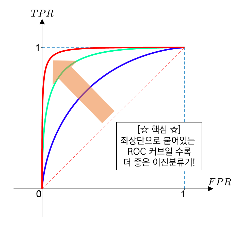
ROC Curve 확인하기
library import
In [115]:
from sklearn.metrics import roc_curve, auc
In [116]:
from sklearn import metrics
AUC 구하기
In [117]:
false_positive_rate, true_positive_rate, thresholds=roc_curve(y_test,model.decision_function(X_scaled_minmax_test))
roc_auc=metrics.roc_auc_score(y_test,model.decision_function(X_scaled_minmax_test))
Out[117]:
0.9923423423423423
In [118]:
roc_auc
Out[118]:
0.9923423423423423
- 결정함수 : 부호를 통해 값 확인 가능
In [120]:
model.decision_function(X_scaled_minmax_test)[1:4]
Out[120]:
array([-3.5070115 , -2.81670291, -3.8601789 ])
ROC Curve 그리기
In [126]:
import matplotlib.pyplot as plt
# title 입력
plt.title("ROC Curve")
# x축
plt.xlabel("False positive rate(1-Specficity)")
# y축
plt.ylabel("True positive rate(Sensitivity)")
# roc curve 그리기
# 색상 지정 : "b"
plt.plot(false_positive_rate,true_positive_rate,"b",label="Model(AUC= %0.2f)"%roc_auc)
# 기준선 그리기
# 선타입/마커 지정
plt.plot([0,1],[1,1],"y--") # (0,1) /(1,1) 지나는 직선, 색상은 yellow
plt.plot([0,1],[0,1],"r--")
plt.legend(loc="lower right")
plt.show()

참고자료 : matplotlib 선/마커 지정하기
선/마커 표시 형식 예시

선/마커 동시 지정하기

설정 방법

예측 결과 정리
train set 예측확률 Dataframe에 저장하기
In [137]:
prob_train=model.predict_proba(X_scaled_minmax_train) # 0,1에 대한 각각의 확률 예측값


y_train[['y_pred']]=pred_train #trainset에 의한 예측 결과 저장

y_train[['y_prob0','y_prob1']]=prob_train
y_train
Out[137]:
| Class | y_pred | y_prob0 | y_prob1 | |
|---|---|---|---|---|
| 131 | 0 | 0 | 0.981014 | 0.018986 |
| 6 | 0 | 0 | 0.768191 | 0.231809 |
| 0 | 0 | 0 | 0.966431 | 0.033569 |
| 269 | 0 | 0 | 0.988880 | 0.011120 |
| 56 | 1 | 1 | 0.203161 | 0.796839 |
| ... | ... | ... | ... | ... |
| 515 | 1 | 1 | 0.021270 | 0.978730 |
| 216 | 1 | 0 | 0.895961 | 0.104039 |
| 312 | 1 | 1 | 0.113440 | 0.886560 |
| 11 | 0 | 0 | 0.987405 | 0.012595 |
| 268 | 0 | 0 | 0.990470 | 0.009530 |
512 rows × 4 columns
In [132]:
pd.DataFrame(prob_train)
Out[132]:
| 0 | 1 | |
|---|---|---|
| 0 | 0.981014 | 0.018986 |
| 1 | 0.768191 | 0.231809 |
| 2 | 0.966431 | 0.033569 |
| 3 | 0.988880 | 0.011120 |
| 4 | 0.203161 | 0.796839 |
| ... | ... | ... |
| 507 | 0.021270 | 0.978730 |
| 508 | 0.895961 | 0.104039 |
| 509 | 0.113440 | 0.886560 |
| 510 | 0.987405 | 0.012595 |
| 511 | 0.990470 | 0.009530 |
512 rows × 2 columns
test set 예측확률 Dataframe에 저장하기
In [138]:
prob_test=model.predict_proba(X_scaled_minmax_test)
y_test[['y_pred']]=pred_test
y_test[['y_prob0','y_prob1']]=prob_test
y_test
Out[138]:
| Class | y_pred | y_prob0 | y_prob1 | |
|---|---|---|---|---|
| 541 | 0 | 0 | 0.955893 | 0.044107 |
| 549 | 0 | 0 | 0.970887 | 0.029113 |
| 318 | 0 | 0 | 0.943572 | 0.056428 |
| 183 | 0 | 0 | 0.979370 | 0.020630 |
| 478 | 1 | 1 | 0.001305 | 0.998695 |
| ... | ... | ... | ... | ... |
| 425 | 1 | 1 | 0.006201 | 0.993799 |
| 314 | 1 | 1 | 0.067440 | 0.932560 |
| 15 | 1 | 1 | 0.436887 | 0.563113 |
| 510 | 0 | 0 | 0.983410 | 0.016590 |
| 351 | 0 | 0 | 0.987405 | 0.012595 |
171 rows × 4 columns
전체 결과 Dataframe으로 병합 후 csv 파일로 저장하기
In [139]:
X_test
Out[139]:
| Clump_Thickness | Cell_Size | Cell_Shape | Marginal_Adhesion | Single_Epithelial_Cell_Size | Bare_Nuclei | Bland_Chromatin | Normal_Nucleoli | Mitoses | |
|---|---|---|---|---|---|---|---|---|---|
| 541 | 5 | 2 | 2 | 2 | 1 | 1 | 2 | 1 | 1 |
| 549 | 4 | 1 | 1 | 1 | 2 | 1 | 3 | 2 | 1 |
| 318 | 5 | 2 | 2 | 2 | 2 | 1 | 2 | 2 | 1 |
| 183 | 1 | 2 | 3 | 1 | 2 | 1 | 3 | 1 | 1 |
| 478 | 5 | 10 | 10 | 10 | 6 | 10 | 6 | 5 | 2 |
| ... | ... | ... | ... | ... | ... | ... | ... | ... | ... |
| 425 | 10 | 4 | 3 | 10 | 4 | 10 | 10 | 1 | 1 |
| 314 | 8 | 10 | 3 | 2 | 6 | 4 | 3 | 10 | 1 |
| 15 | 7 | 4 | 6 | 4 | 6 | 1 | 4 | 3 | 1 |
| 510 | 3 | 1 | 1 | 2 | 2 | 1 | 1 | 1 | 1 |
| 351 | 2 | 1 | 1 | 1 | 2 | 1 | 2 | 1 | 1 |
171 rows × 9 columns
In [140]:
y_test
Out[140]:
| Class | y_pred | y_prob0 | y_prob1 | |
|---|---|---|---|---|
| 541 | 0 | 0 | 0.955893 | 0.044107 |
| 549 | 0 | 0 | 0.970887 | 0.029113 |
| 318 | 0 | 0 | 0.943572 | 0.056428 |
| 183 | 0 | 0 | 0.979370 | 0.020630 |
| 478 | 1 | 1 | 0.001305 | 0.998695 |
| ... | ... | ... | ... | ... |
| 425 | 1 | 1 | 0.006201 | 0.993799 |
| 314 | 1 | 1 | 0.067440 | 0.932560 |
| 15 | 1 | 1 | 0.436887 | 0.563113 |
| 510 | 0 | 0 | 0.983410 | 0.016590 |
| 351 | 0 | 0 | 0.987405 | 0.012595 |
171 rows × 4 columns
In [147]:
# pd.concat : dataframe 합치기
# axis=0 (기본값) : 열을 추가 (세로 병합)
# axis=1 : 변수를 합침 (가로 병합)
# Total_test=pd.concat([X_test,y_test],axis-1)
Total_test=pd.concat([X_test,y_test], axis=1)
# csv로 내보내기
Total_test.to_csv("classification_logistic.csv")
In [149]:
Total_test.head(20)
Out[149]:
| Clump_Thickness | Cell_Size | Cell_Shape | Marginal_Adhesion | Single_Epithelial_Cell_Size | Bare_Nuclei | Bland_Chromatin | Normal_Nucleoli | Mitoses | Class | y_pred | y_prob0 | y_prob1 | |
|---|---|---|---|---|---|---|---|---|---|---|---|---|---|
| 541 | 5 | 2 | 2 | 2 | 1 | 1 | 2 | 1 | 1 | 0 | 0 | 0.955893 | 0.044107 |
| 549 | 4 | 1 | 1 | 1 | 2 | 1 | 3 | 2 | 1 | 0 | 0 | 0.970887 | 0.029113 |
| 318 | 5 | 2 | 2 | 2 | 2 | 1 | 2 | 2 | 1 | 0 | 0 | 0.943572 | 0.056428 |
| 183 | 1 | 2 | 3 | 1 | 2 | 1 | 3 | 1 | 1 | 0 | 0 | 0.979370 | 0.020630 |
| 478 | 5 | 10 | 10 | 10 | 6 | 10 | 6 | 5 | 2 | 1 | 1 | 0.001305 | 0.998695 |
| 65 | 5 | 3 | 4 | 1 | 8 | 10 | 4 | 9 | 1 | 1 | 1 | 0.049745 | 0.950255 |
| 430 | 2 | 1 | 1 | 1 | 2 | 1 | 1 | 1 | 1 | 0 | 0 | 0.989204 | 0.010796 |
| 17 | 4 | 1 | 1 | 1 | 2 | 1 | 3 | 1 | 1 | 0 | 0 | 0.974468 | 0.025532 |
| 443 | 5 | 1 | 2 | 1 | 2 | 1 | 1 | 1 | 1 | 0 | 0 | 0.969380 | 0.030620 |
| 77 | 2 | 1 | 1 | 1 | 3 | 1 | 2 | 1 | 1 | 0 | 0 | 0.985760 | 0.014240 |
| 212 | 6 | 10 | 7 | 7 | 6 | 4 | 8 | 10 | 2 | 1 | 1 | 0.009908 | 0.990092 |
| 95 | 5 | 1 | 1 | 1 | 2 | 1 | 3 | 1 | 1 | 0 | 0 | 0.966431 | 0.033569 |
| 659 | 4 | 1 | 4 | 1 | 2 | 1 | 1 | 1 | 1 | 0 | 0 | 0.964539 | 0.035461 |
| 143 | 1 | 1 | 1 | 1 | 3 | 2 | 2 | 1 | 1 | 0 | 0 | 0.984538 | 0.015462 |
| 383 | 4 | 1 | 1 | 1 | 2 | 1 | 1 | 1 | 1 | 0 | 0 | 0.981179 | 0.018821 |
| 560 | 5 | 1 | 2 | 1 | 2 | 1 | 3 | 1 | 1 | 0 | 0 | 0.958638 | 0.041362 |
| 634 | 3 | 1 | 1 | 2 | 3 | 4 | 1 | 1 | 1 | 0 | 0 | 0.945899 | 0.054101 |
| 311 | 3 | 2 | 2 | 1 | 2 | 1 | 2 | 3 | 1 | 0 | 0 | 0.967679 | 0.032321 |
| 451 | 10 | 6 | 6 | 2 | 4 | 10 | 9 | 7 | 1 | 1 | 1 | 0.003909 | 0.996091 |
| 117 | 3 | 2 | 1 | 1 | 2 | 2 | 3 | 1 | 1 | 0 | 0 | 0.966576 | 0.033424 |
pd.concat axis=1,axis=0 차이
In [146]:
pd.concat([X_test,y_test], axis=0)
Out[146]:
| Clump_Thickness | Cell_Size | Cell_Shape | Marginal_Adhesion | Single_Epithelial_Cell_Size | Bare_Nuclei | Bland_Chromatin | Normal_Nucleoli | Mitoses | Class | y_pred | y_prob0 | y_prob1 | |
|---|---|---|---|---|---|---|---|---|---|---|---|---|---|
| 541 | 5.0 | 2.0 | 2.0 | 2.0 | 1.0 | 1.0 | 2.0 | 1.0 | 1.0 | NaN | NaN | NaN | NaN |
| 549 | 4.0 | 1.0 | 1.0 | 1.0 | 2.0 | 1.0 | 3.0 | 2.0 | 1.0 | NaN | NaN | NaN | NaN |
| 318 | 5.0 | 2.0 | 2.0 | 2.0 | 2.0 | 1.0 | 2.0 | 2.0 | 1.0 | NaN | NaN | NaN | NaN |
| 183 | 1.0 | 2.0 | 3.0 | 1.0 | 2.0 | 1.0 | 3.0 | 1.0 | 1.0 | NaN | NaN | NaN | NaN |
| 478 | 5.0 | 10.0 | 10.0 | 10.0 | 6.0 | 10.0 | 6.0 | 5.0 | 2.0 | NaN | NaN | NaN | NaN |
| ... | ... | ... | ... | ... | ... | ... | ... | ... | ... | ... | ... | ... | ... |
| 425 | NaN | NaN | NaN | NaN | NaN | NaN | NaN | NaN | NaN | 1.0 | 1.0 | 0.006201 | 0.993799 |
| 314 | NaN | NaN | NaN | NaN | NaN | NaN | NaN | NaN | NaN | 1.0 | 1.0 | 0.067440 | 0.932560 |
| 15 | NaN | NaN | NaN | NaN | NaN | NaN | NaN | NaN | NaN | 1.0 | 1.0 | 0.436887 | 0.563113 |
| 510 | NaN | NaN | NaN | NaN | NaN | NaN | NaN | NaN | NaN | 0.0 | 0.0 | 0.983410 | 0.016590 |
| 351 | NaN | NaN | NaN | NaN | NaN | NaN | NaN | NaN | NaN | 0.0 | 0.0 | 0.987405 | 0.012595 |
342 rows × 13 columns
In [ ]:
'빅데이터분석기사 자료 > 2) 빅.분. 기 - ML' 카테고리의 다른 글
| [빅.분.기] 작업형2유형 - 랜덤포레스트 (0) | 2022.02.23 |
|---|---|
| [빅.분.기] 작업형2유형 - 문제 연습 (0) | 2022.01.08 |
| [빅.분.기] 작업형2유형 - Train/Test 셋 분리 (0) | 2022.01.08 |
| [빅.분.기] 작업형2유형 - One Hot Encoding (0) | 2022.01.08 |
댓글